PyMacLab Tutorial Series¶

Tutorial 1 - Getting started¶

Introduction¶

PyMacLab’s strength or orginal design goal has been that of providing users with a rich and flexible DSGE data structure (also called class in object-oriented programming speak) which allows them to do lots of interesting things with DSGE models. Don’t forget that another stated goal of PyMacLab is to permit researchers to work with DSGE models who know how to and enjoy to use the programming language Python. This tutorial assumes that you already know how to use Python, if you are completely new to it I suggest you consult one of the many tutorials available on the internet to get started with the language. Don’t forget that Python is free as in free as freedom, no proprietary software such as Matlab is tainting the freedom of the environment you will be working in when using PyMacLab.

The easiest and best way to get started and explore all of the available features of PyMacLab, or for that matter any other Python library, is to work with IPython, which is an abbreviation for Interactive Python. With this program, Python users who are scientifically inclined, can more or less emulate the behaviour of programs such as Matlab, Octave or Scilab. This means that sessions can be launched in which commands entered into a command prompt are executed immediately and resulting output is printed to screen. It also means that generated objects resulting from such computations carried out at the command prompt (such as matrices or DSGE models) begin to exist within the session’s variable scope and become ready for further manipulation, i.e. they persist. Before being able to work with PyMacLab we have to launch an IPython session and import the library into it’s scope:
# Import the pymaclab module into its namespace
In [1]: import pymaclab as pm

# Get the version and author's name
In [2]: pm.__version__
'0.95.1'

# Get the library's author's name
In [3]: pm.__author__
'Eric M. Scheffel'
Here we simply have imported the PyMacLab module and inspected some of its attributes, such as the current version numbering as well as them module’s author’s name. Let’s look deeper into the recesses of the module though to better understand who it is organized
# Import the pymaclab module into its namespace
In [1]: import pymaclab as pm

# Use the dir() command to view all available attributes and method calls,
# this command returns a list
In [2]: dir(pm)
['OPS',
'__builtins__',
'__doc__',
'__file__',
'__name__',
'__package__',
'__path__',
'dattrans',
'db_graph',
'dsge',
'explain',
'favar',
'filters',
'ldbs',
'linalg',
'lmods',
'lvars',
'macrolab',
'make_modfile',
'modedit',
'modfiles',
'modinfo',
'modsolve',
'newDB',
'newFAVAR',
'newMOD',
'newVAR',
'pyed',
'stats',
'sys',
'texedit',
'var']
As you can see the module contains a quite a few attributes, many of which are still experimental and perhaps best not called at this stage. The most mature and arguable most interesting method call is that called pm.newMOD, which allows users to instantiate a DSGE model instance, which would be done like so:
# Import the pymaclab module into its namespace, also import os module
In [1]: import pymaclab as pm
In [2]: import os

# Define the relative path to your modfiles
In [3]: modpath = "../pymaclab/modfiles/models/stable"

# Instantiate a new DSGE model instance like so
In [4]: rbc1 = pm.newMOD(os.path.join(modpath,"rbc1_res.txt"))

# As an example, check the models computed steady stated
In [5]: print rbc1.sstate
{'betta': 0.99009900990099009,
'c_bar': 2.7560505909330626,
'k_bar': 38.160700489842398,
'y_bar': 3.7100681031791227}
Alternatively, you can also test some of the DSGE model files which come supplied with PyMacLab’s standard installation. For this to work all you have to do is to import a provided handler module, pymaclab.modfiles.models, which contains all of the DSGE models’ names and their correspoding full file paths. Notice however that the models themselves are further classified into three categories, models.stable, models.testing and models.development which helps to distinguish between models which are in the process of being added and such which are known to work correctly:
 # Import the pymaclab module into its namespace, also import os module
 In [1]: import pymaclab as pm
 # Import the DSGE models' filepath handle
 In [2]: from pymaclab.modfiles import models

 #Check all of the available models in the stable branch
 In [3]: dir(models.stable)
 ['__builtins__',
 '__doc__',
 '__file__',
 '__name__',
 '__package__',
 '__path__',
 'jermann98',
 'jermann98_ext',
 'merz',
 'prog',
 'rbc1_cf',
 'rbc1_ext',
 'rbc1_extss',
 'rbc1_focs',
 'rbc1_num',
 'rbc1_res',
 'rbc1_sug',
 'rbc2',
 'sims']

 #Check all of the available models in the development branch
 In [4]: dir(models.development)
['RBC_Romer',
 '__builtins__',
 '__doc__',
 '__file__',
 '__name__',
 '__package__',
 '__path__',
 'max1',
 'max2',
 'mbc1',
 'model2',
 'model3',
 'nk_nocapital',
 'nkm',
 'nkm_nocapital']

 #Check all of the available models in the testing branch
 In [5]: dir(models.testing)
 ['__builtins__',
 '__doc__',
 '__file__',
 '__name__',
 '__package__',
 '__path__',
 'cee']


 # The DSGE models objects in pymaclab.modfiles.models
 # are just references to full file paths, i.e.

 In [6]: models.stable.rbc1_res
 '/usr/lib/python2.7/site-packages/pymaclab/modfiles/rbc1_res.txt'

 #Instantiate a new DSGE model instance like so
 In [7]: rbc1 = pm.newMOD(models.stable.rbc1_res)

 #As an example, check the models computed steady stated
 In [8]: print rbc1.sstate
 {'betta': 0.99009900990099009,
 'c_bar': 2.7560505909330626,
 'k_bar': 38.160700489842398,
 'y_bar': 3.7100681031791227}
Now we have already seen some of the power and simplicity we can leverage by using PyMacLab. Before learning some of its additional power, we do however still need to take a quick detour to study the model file rbc1.txt which we had to pass as an argument to the pm.newMOD method call, as its structure is determined by a set of conventions which are important to adhere to in order to enable PyMacLab to parse and employ the information contained therein correctly and efficiently.

Tutorial 3 - The PyMacLab DSGE instance¶

Introduction¶

As already stated in the introduction of the introductory basic tutorial, PyMacLab’s strength or orginal design goal has been that of providing users with a rich and flexible DSGE data structure (also called Class in object-oriented programming speak) which allows them to do lots of interesting things with DSGE models and to treat them as if they were some kind of primitive data type in their own right. While the previous tutorial described some basics as well as the all-important DSGE model file structure and syntax conventions, in this section I am going to stress some of the object-oriented programming features of PyMacLab, in particular the structure of a PyMacLab DSGE model instance or data structure.

Readers with a background in modern programming languages supporting the object-oriented programming (OOP) paradigm will easily relate to concepts in this sections, while for others it may appear more cryptic at first sight. But to convey these concepts to researchers is important, as it stresses many particular advantages of PyMacLab over other programs, and in particular its flexibility, transparency, consistency, persistence and enormous scope for extensibility. All example code fragments provided here assume that you are replicating them within an IPyton interactive session, but they could also be called from a Python program “batch” file.

Understanding the PyMacLab DSGE model class and its instances¶

PyMacLab has been written in the Python programming language which supports object-oriented programming. This means, that more than 80% of PyMacLab’s code is devoted to the definition of data fields and methods of the DSGE_model Class, which forms the basis for all DSGE models users can load, spawn or instantiate and interact with once they have imported they PyMacLab library into their programs. As already explained elsewhere, the basis of all DSGE model instances is the DSGE model’s model text file in which it is defined in terms of its specific characteristics, such as its parameters and first-order conditions of optimality. We recall that this process of loading or instantiating a DSGE model worked as follows:
# Import the pymaclab module into its namespace, also import os module
In [1]: import pymaclab as pm
In [2]: from pymaclab.modfiles import models

# Instantiate a new DSGE model instance like so
In [4]: rbc1 = pm.newMOD(models.stable.rbc1)
After executing these lines of code in an interactive environment such as that provided by IPython, which emulates well the feel and behaviour of the Matlab interactive environment, the DSGE instance or data object going by the name of rbc1 now exists in the namespace of the running program and can be put to further use. But before looking at these various ways possible to make effective use of this DSGE model instance, let’s first trace the various steps the programs goes through when a DSGE model get instantiated. So what happens internally when the above last line in the code fragment is called:

The empty shell DSGE model instance gets instantiated

The DSGE model instance reads the model file provided to it and any other arguments and saves them by attaching them to itself.

Instantiation Step 1: The files get read in and a method defined on the instance simply splits the file into its individual sections and saves these raw sections by attaching them to itself.

Instantiation Step 2: A parser method is called which disaggregates the raw information provided in each section of the model file and begins to extract meaningful information from it, each time saving this information by attaching it to itself as data fields. Also, the DSGE model instance is prepared and set up in order to attempt to solve for the steady state of it manually at the command line, instead of doing it automatically. If you want the model instance to do ONLY this next step and stop there for you to explore further interactively, you must call the command with and extra argument like this:
# Import the pymaclab module into its namespace, also import os module
In [1]: import pymaclab as pm
In [2]: from pymaclab.modfiles import models

# Instantiate a new DSGE model instance like so, but adding initlev=0 as extra argument
In [3]: rbc1 = pm.newMOD(models.stable.rbc1,initlev=0)
Instantiation Step 3: The information is used in order to attempt to compute the numerical steady-state of the model. If you want the model instance to do ONLY this next step and stop there for you to explore further interactively, you must call the command with and extra argument like this:
# Import the pymaclab module into its namespace, also import os module
In [1]: import pymaclab as pm
In [2]: from pymaclab.modfiles import models

# Instantiate a new DSGE model instance like so, but adding initlev=1 as extra argument
In [3]: rbc1 = pm.newMOD(models.stable.rbc1,initlev=1)
Instantiation Step 4: If the steady state was computed successfully then the model’s analytical and numerical Jacobian and Hessian are computed. Finally a preferred dynamic solution method is called which solves the model for its policy function and other laws of motion.

To give users a choice of “solution depths” at DSGE object instantiation time is important and useful, especially in the initial experimentation phase during which the DSGE model file gets populated. That way researchers can first carefully solve one part of the problem (i.e. looking for the steady state) and indeed choose to do so manually on the IPython interactive command shell, allowing them to immediately inspect any errors.

Instantiation options for DSGE model instances¶

There are a couple of instance invocation or instantiation arguments one should be aware of. At the time of writing these lines there are in total 5 other arguments (besides the DSGE model template file path) which can be passed to the pymaclab.newMOD function out of which 1 is currently not (yet) supported and not advisable to employ. The other 4 options determine the initiation level of the DSGE model (i.e. how far it should be solved if at all), whether diagnosis messages should be printed to screen during instantiation, how many CPU cores to employ when building the Jacobian and Hessian of the model, and finally whether the expensive-to-compute Hessian should be computed at all. Remember that the last option is useful as many researchers often - at least initially - want to explore the solution to their model to a first order of approximation before taking things further. So here are the options again in summary with their default values:

Option with default value Description

pm.newMOD(mpath,initlev=2) Initlev=0 only parses and prepares for manual steady state calculation

Initlev=1 does initlev=0 and attempts to solve for the model’s steady state automatically

Initlev=2 does initlev=0, initlev=1 and generates Jacobian and Hessian and solves model dynamically

pm.newMOD(mpath,mesg=False) Prints very useful runtime instantiation messages to the screen for users to follow progress

pm.newMOD(mpath,ncpus=1) CPU cores to be used in expensive computation of model’s derivatives, ‘auto’ for auto-detection

pm.newMOD(mpath,mk_hessian=True) Should Hessian be computed at all, as is expensive?

pm.newMOD(mpath,use_focs=False) Should only the model’s FOCs be used to computed the steady state? Accepts Python list or tuple

pm.newMOD(mpath,ssidic=None) Use in conjunction with previous argument to specify initial starting values as Python dictionary

pm.newMOD(mpath,sstate=None) Specify steady state values as Python dictionary and supply here. No SS computation in instance

Needless to say, all of the options can be and usually are called in combination, they are only shown separately here for sake of expositional clarity. Medium-sized to large-sized models can take considerable time to compute the Jacobian alone, let alone the Hessian. On the other hand passing more (real as opposed to virtual) CPU cores to the instantiation process can significantly cut down computation time. In this case, the FOCs nonlinear equations are distributed to individual cores for analytical differentiation as opposed to doing this serially on one CPU core.

Working with DSGE model instances¶

The most useful feature is to call the model with the option initlev=0, because this will allow you more control over the steady-state computation of the model by permitting a closer interactive inspection of the DSGE model instance as created thus far. Let’s demonstrate this here:
# Import the pymaclab module into its namespace, also import os module
In [1]: import pymaclab as pm
In [2]: from pymaclab.modfiles import models

# Instantiate a new DSGE model instance like so, but adding initlev=0 as extra argument
In [3]: rbc1 = pm.newMOD(models.stable.rbc1,initlev=0)

# This datafield contains the original nonlinear system expressed as g(x)=0
In [4]: rbc1.sssolvers.fsolve.ssm
['z_bar*k_bar**(rho)-delta*k_bar-c_bar',
 'rho*z_bar*k_bar**(rho-1)+(1-delta)-R_bar',
 '(betta*R_bar)-1',
 'z_bar*k_bar**(rho)-y_bar']

# This datafield contains the initial values supplied to the rootfinder algorithm
In [5]: rbc1.sssolvers.fsolve.ssi
{'betta': 1.0, 'c_bar': 1.0, 'k_bar': 1.0, 'y_bar': 1.0}

# Instead of letting the model during instantiation solve the model all the way through,
# we can solve for the steady state by hand, manually
In [6]: rbc1.sssolvers.fsolve.solve()

# And then inspect the solution and some message returned by the rootfinder
In [6]: rbc1.sssolvers.fsolve.fsout
{'betta': 0.9900990099009901,
 'c_bar': 2.7560505909330626,
 'k_bar': 38.1607004898424,
 'y_bar': 3.7100681031791227}

In [7]: rbc1.sssolvers.fsolve.mesg
'The solution has converged.'
Another useful lesson to take away from this example is that a DSGE model instance is like a many-branch tree structure, just like the Windows File Explorer so many people are familiar with, where individual “nodes” represent either data fields or methods (function calls) which equip the model instance with some functionality. This kind of approach of structuring and programming a solution to the problem of designing a program which handles the solution-finding of DSGE models offers enormous scope for experimentation and extensibility. After a DSGE model has been instantiated without passing the initlev argument, you can inspect this structure like so:
# Import the pymaclab module into its namespace, also import os module
In [1]: import pymaclab as pm
In [2]: from pymaclab.modfiles import models

# Instantiate a new DSGE model instance like so
In [3]: rbc1 = pm.newMOD(models.stable.rbc1)

# Inspect the data fields and methods of the DSGE model instance
In [4]: dir(rbc1)
['__class__',
 '__delattr__',
 '__dict__',
 '__doc__',
 '__format__',
 '__getattribute__',
 '__hash__',
 '__init__',
 '__module__',
 '__new__',
 '__reduce__',
 '__reduce_ex__',
 '__repr__',
 '__setattr__',
 '__sizeof__',
 '__str__',
 '__subclasshook__',
 '__weakref__',
 '_initlev',
 'audic',
 'author',
 'ccv',
 'dbase',
 'deltex',
 'getdata',
 'info',
 'init2',
 'manss_sys',
 'mkeigv',
 'mkjahe',
 'mkjahen',
 'mkjahenmat',
 'mkjahepp',
 'mkjaheppn',
 'mod_name',
 'modfile',
 'nall',
 'ncon',
 'nendo',
 'nexo',
 'nlsubs',
 'nlsubs_list',
 'nlsubs_raw1',
 'nlsubs_raw2',
 'nother',
 'nstat',
 'numssdic',
 'paramdic',
 'pdf',
 'setauthor',
 'ssidic',
 'sssolvers',
 'sstate',
 'ssys_list',
 'subs_vars',
 'switches',
 'texed',
 'txted',
 'txtpars',
 'updf',
 'updm',
 'vardic',
 'vreg']
As you can see, the attributes exposed at the root of the instance are plenty and can be acccessed in the usual way:
# Import the pymaclab module into its namespace, also import os module
In [1]: import pymaclab as pm
In [2]: from pymaclab.modfiles import models

# Instantiate a new DSGE model instance like so
In [3]: rbc1 = pm.newMOD(models.stable.rbc1)

# Access one of the model's fields
In [4]: rbc1.ssys_list
['z_bar*k_bar**(rho)-delta*k_bar-c_bar',
'rho*z_bar*k_bar**(rho-1)+(1-delta)-R_bar',
'(betta*R_bar)-1',
'z_bar*k_bar**(rho)-y_bar']
So one can observe that the data field rbc1.ssys_list simply summarizes the system of nonlinear equations which has been described in the relevant section of the DSGE model file. Now you know how to explore the DSGE model instance and understand its general structure, and we conclude this short tutorial by inviting you to do so. Don’t forget that some nodes at the root possess further sub-nodes, as was the case when cascading down the rbc1.sssolvers branch. To help your search, the only other node with many more sub-nodes is the rbc1.modsolvers branch, which we will explore more in the next section to this tutorial series.

DSGE modelling made intuitive¶

Before concluding this tutorial, we will demonstrate how PyMacLab’s DSGE data structure (or instance) approach allows researchers to implement ideas very intuitively, such as for instance “looping” over a DSGE model instance in order to explore how incremental changes to the parameter space alter the steady state of the model. Leaving our usual interactive IPyton shell, consider the following Python program file:
# Import the pymaclab module into its namespace
# Also import Numpy for array handling and Matplotlib for plotting
import pymaclab as pm
from pymaclab.modfiles import models
import numpy as np
from matplotlib import pyplot as plt

# Instantiate a new DSGE model instance like so
rbc1 = pm.newMOD(models.stable.rbc1)

# Create an array representing a finely-spaced range of possible impatience values
# Then convert to corresponding steady state gross real interest rate values
betarr = np.arange(0.8,0.99,0.001)
betarr = 1.0/betarr

# Loop over the RBC DSGE model, each time re-computing for new R_bar
ss_capital = []
for betar in betarr:
    rbc1.updaters.paramdic['R_bar'] = betar # assign new R_bar to model
    rbc1.sssolvers.fsolve.solve() # re-compute steady stae
    ss_capital.append(rbc1.sssolvers.fsolve.fsout['k_bar']) # fetch and store k_bar

# Create a nice figure
fig1 = plt.figure()
plt.grid()
plt.title('Plot of steady state physical capital against R\_bar')
plt.xlabel(r'Steady state gross real interest rate')
plt.ylabel(r'Steady State of physical capital')
plt.plot(betarr,ss_capital,'k-')
plt.show()
Anybody who has done some DSGE modelling in the past will easily be able to intuitively grasp the purpose of the above code snippet. All we are doing here is to loop over the same RBC model, each time feeding it with a slightly different steady state groos real interest rate value and re-computing the steady state of the model. This gives rise to the following nice plot exhibting the steady state relationship between the interest rate and the level of physical capital prevailing in steady state:

(Source code, png, hires.png, pdf)

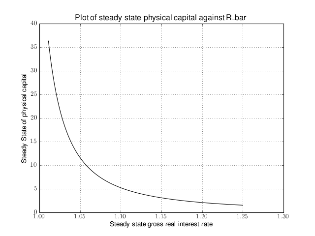
That was nice and simple, wasn’t it? So with the power and flexibility of PyMacLab DSGE model instances we can relatively painlessly explore simple questions such as how differing deep parameter specifications for the impatience factor $\beta$ can affect the steady state level of physical capital. And indeed, as intuition would suggest, less patient consumers are less thrifty and more spend-thrifty thus causing a lower steady state level of physical capital in the economy. This last example also serves to make another important point. PyMacLab is not a program such as Dynare, but instead an add-in library for Python prividing an advanced DSGE model data structure in form of a DSGE model class which can be used in conjunction with any other library available in Python.

Tutorial 4 - The Python DSGE instance updater methods¶

Introduction¶

In the previous tutorial we described the general structure and some of the behaviour of PyMacLab’s DSGE model’s object-oriented design and what kind of advantages model builders can derive from this. In particular, at the end of the last tutorial, we saw how the decision to design DSGE model’s instances essentially in from of an object-oriented advanced data structure with well-defined data fields and methods allowed us to “loop over” a DSGE model instance many times over, each time feeding the instance with slightly a different value for the impatience factor $\beta$ and obtaining a new value for the corresponding steady state value of physical capital.

To be able to do something like this simply and intuitively is one of the many advantages that PyMacLab has over traditional DSGE model solving programs such as Dynare. While Dynare is a complete program allowing users to solve for specific DSGE models with little added post-solution programmatic flexibility, PyMacLab is from ground up designed to be a library providing an object-oriented Class-defined advanced data structure with data fields and behaviour in form of methods. This makes it incredibly easy to build programs which treat DSGE models as if they were simple data structures, such as integers, floats, lists or any other data structure you are familiar with from using a number of different programming languages. This makes PyMacLab incredibly flexible for within- and post-solution program interventions, where in this section we will define more clearly what we meant by program interventions. The main point to take away from all of this is that Dynare is a canned program to get specific solutions, while PyMacLab is a Python plugin library, whose only purpose is to make available an advanced DSGE model class suitable for carrying out a variety of tasks.

While in programs like Dynare the most important aspect from the point of view of model builders to obtaining the solution of DSGE models lies in the specification of so-called model files, the proper way to understand the more flexible operation of PyMacLab is to view the model template only as a specific point of departure from which to start your analysis from. The only point of making use of model template files is to initialize or instantiate a DSGE model instance, the real power in using PyMacLab lies in the methods made available to researchers which become available after model files have been read in and the DSGE model instances become available inside the Python interactive environment. It is this post-instantiation scope for activity and alteration which makes using PyMacLab so much fun for researchers. As already illustrated in the previous tutorial, this design decision opens up the possibility of easily and intuitively obtaining a large permutation of possible solution outcomes quickly. There are two convenience methods or avenues open to the researcher to intelligently update DSGE model instances dynamically at runtime which we will describe in some detail next.

One-off alteration of one specific model property¶

Once a DSGE model is instantiated using a model template files as a point of departure and a specific source of information from which model properties get parsed and attached as data fields to the DSGE model instance, all we have done is to initialize or read into memory a specific state of our DSGE model. You may also recall that the nature of this state differs crucially depending upon what kind of initlev parameter value was passed at DSGE model instantiation. So we recall that at initlev=0 only information gets parsed in but nothing at all gets solved, not even the steady state. Other values for initlev gave rise to instantiated model instances which were solved all down to ever deeper levels including possibly including the steady state and dynamic elasticities (policy functions). In this section I will briefly describe methods allowing a functionality akin to comparative statics analysis in PyMacLab in which models can get easily be re-initialized with different model information injected into existing DSGE model instances dynamically at runtime.

One way of using PyMacLab to carry out a kind of comparative statics analysis has already been touched upon for one specific case in the previous tutorial, using the example of the rbc1.updaters.paramdic attribute. In general you will discover that navigating into the rbc1.updaters. branch of the model exposes a number of data fields which in exact name are also available at the root rbc1. of the model. So how then does rbc1.updaters.paramdic differ from its counterpart available at the root rbc1.paramdic?

The answer to this question is that while rbc1.paramdic is just the parameter dictionary which get populated at model instantiation time, rbc1.updaters.paramdic is a “wrapped” version of the same dictionary with the added behaviour that if a new values gets inserted into it using the relevant dictionary methods, such as rbc1.updaters.paramdic['R_bar']=1.02 or rbc1.updates.paramdic.update(dic_alt) where dic_alt is some other dictionary containing updated values of one or more keyed item in the original paramdic, then an internal function gets triggered at assignment time which re-initializes the model using the updated values for paramdic.

If the newly assigned value is exactly identical to the value which was already stored in the original paramdic, then the model will not get updated as its state has remained unaltered. The following smart one-off updaters are available all of which possess the above described behaviour. Notice also that the DSGE model will only get updated down to the level first specified in initlev at model instantiation time. Also, when any of these wrapped updater objects just gets called in the normal way they behave exactly as their non-wrapped counterparts by returning the values stored in them without any additional behaviour updating the model.

Wrapped updater object Description

model.updaters.paramdic Inserting updated values re-initializes the model with new set of parameter values

model.updaters.vardic Inserting new values updates/changes values and attributes defined for variables used in the model

model.updaters.nlsubsdic Inserting new values updates the dictionary of variable substitution items beginning with @

model.updaters.foceqs Inserting new string equations updates the set of non-linear first-order conditions of optimality

model.updaters.manss_sys In this list users can insert new equations as strings into the closed form steady state system

model.updaters.ssys_list In this list users can insert new equations as strings into the numerical steady state system

model.updaters.sigma A wrapped matrix which updates the model when changed values are inserted in the varcovar-matrix

Notice how in this branch rbc1.updaters. changing wrapped objects by assigning new values will trigger automatic updating of the DSGE model immediately upon assignment. This behaviour may not always be desirable whenever a series of changes need to be made before updating of the model can be considered. Whenever such situations occur an alternative route needs to be taken which we will explore next.

Altering many model properties and queued processing¶

At times researchers may want to load or instantiate a particular DSGE model instance using a corresponding template file but then perhaps plan to radically modify the model dynamically at runtime, by combining such actions as introducing new time-subscripted variables, altering the deep parameter space and adding new or augmenting existing equations in the system of non-linear FOCs. Whenever such radical alterations are considered, they will often have to happen in combindation before the model gets updated using the new information passed to it. In this case users will use the same wrapped objects already described above but instead use them in the rbc1.updaters_queued. branch.

Here, first a number of changes can be made to objects such as rbc1.updaters_queued.paramdic or rbc1.updaters_queued.foceqs, etc. which by themselves will not trigger an automatic model updating functionality. Instead all changes will be put into a queue which will then have to be processed manually by calling the method rbc1.updaters_queued.process_queue() after all desired changes have been made. This addscenormous flexibility to model builders’ options, as they can essentially build a completely new model at runtime dynamically starting from a simple model instantiated at the outset of their Python scripts/batch files. Therefore, this functionality allows users to dynamically update all information at runtime which was first parsed from the model template file, each time re-computing the DSGE model’s new state given the changes made after the call to the queue processing method has been made.

Wrapped updater object Description

model.updaters_queued.paramdic Inserting updated values re-initializes the model with new set of parameter values

model.updaters_queued.vardic Inserting new values updates/changes values and attributes defined for variables used in the model

model.updaters_queued.nlsubsdic Inserting new values updates the dictionary of variable substitution items beginning with @

model.updaters_queued.foceqs Inserting new string equations updates the set of non-linear first-order conditions of optimality

model.updaters_queued.manss_sys In this list users can insert new equations as strings into the closed form steady state system

model.updaters_queued.ssys_list In this list users can insert new equations as strings into the numerical steady state system

model.updaters_queued.sigma A wrapped matrix which updates the model when changed values are inserted in the varcovar-matrix

model.updaters_queued.queue The actual queue. Here objects which have been altered will be stored as strings

model.updaters_queued.process_queue The queue processing method which finally updates the queued objects in the right order

Tutorial 5 - Steady State Solution Methods¶

Introduction¶

In the previous tutorial we learnt how a PyMacLab DSGE model instance possesses the capability to intelligently upate its properties following the re-declaration at runtime of attached data fields such as the parameter space or the set of non-linear first-order conditions of optimality. In this section we will learn an important component to PyMacLab’s DSGE models which provides users with a large number of options available for solving models’ steady state solution. The great number of possible avenues to take here is quite deliberate; it would be reasonable to argue that for medium- to large-sized models the most difficult part to finding the general dynamic solution based on the approximation method of perturbations is to first obtain the steady state solution around which the approximations are computed. In total we are going to explore 7 different variants suitable for seeking to compute the steady state. So let’s get started.

Option 1: Using the model’s declared FOCs and passing arguments at model instantiation¶

Choosing option 1 allows users to leave the numerical as well as closed form steady state sections in the model template files entirely empty or unused indicated by the “None” keyword inserted into any line in these sections. In this case, the library has to rely on the time- subscripted non-linear first-order conditions of optimality, convert them to steady state equivalents and somehow discover the required set of initial guesses for the variables’ steady states to be searched for using the non-linear root-finding algorithm. This is accomplised in the following way. Consider first the following simple example of a DSGE model file:
%Model Description+++++++++++++++++++++++++++++++++++++++++++++++++++++++++++++++++++++
This is just a standard RBC model, as you can see.


%Model Information+++++++++++++++++++++++++++++++++++++++++++++++++++++++++++++++++++++
Name = Standard RBC Model;


%Parameters++++++++++++++++++++++++++++++++++++++++++++++++++++++++++++++++++++++++++++
rho       = 0.36;
delta     = 0.025;
R_bar     = 1.01;
betta     = 1/R_bar;
eta       = 2.0;
psi       = 0.95;
z_bar     = 1.0;
sigma_eps = 0.052;


%Variable Vectors+++++++++++++++++++++++++++++++++++++++++++++++++++++++++++++++++++++++
[1]  k(t):capital{endo}[log,bk]
[2]  c(t):consumption{con}[log,bk]
[4]  y(t):output{con}[log,bk]
[5]  z(t):eps(t):productivity{exo}[log,bk]
[6]  @inv(t):investment[log,bk]
[7]  @R(t):rrate

%Boundary Conditions++++++++++++++++++++++++++++++++++++++++++++++++++++++++++++++++++++
None


%Variable Substitution Non-Linear System++++++++++++++++++++++++++++++++++++++++++++++++
[1]   @inv(t)   = k(t)-(1-delta)*k(t-1);
[2]   @inv_bar  = SS{@inv(t)};
[3]   @F(t)     = z(t)*k(t-1)**rho;
[4]   @F_bar    = SS{@F(t)};
[5]   @R(t)     = 1+DIFF{@F(t),k(t-1)}-delta;
[6]   @R_bar    = SS{@R(t)};
[7]   @R(t+1)   = FF_1{@R(t)};
[8]   @U(t)     = c(t)**(1-eta)/(1-eta);
[9]   @MU(t)    = DIFF{@U(t),c(t)};
[10]  @MU(t+1)  = FF_1{@MU(t)};



%Non-Linear First-Order Conditions++++++++++++++++++++++++++++++++++++++++++++++++++++++
# Insert here the non-linear FOCs in format g(x)=0

[1]   @F(t)-@inv(t)-c(t) = 0;
[2]   betta*(@MU(t+1)/@MU(t))*@R(t+1)-1 = 0;
[3]   @F(t)-y(t) = 0;
[4]   LOG(E(t)|z(t+1))-psi*LOG(z(t)) = 0;


%Steady States [Closed Form]+++++++++++++++++++++++++++++++++++++++++++++++++++++++++++++
None


%Steady State Non-Linear System [Manual]+++++++++++++++++++++++++++++++++++++++++++++++++
None


%Log-Linearized Model Equations++++++++++++++++++++++++++++++++++++++++++++++++++++++++++
None


%Variance-Covariance Matrix++++++++++++++++++++++++++++++++++++++++++++++++++++++++++++++
Sigma = [sigma_eps**2];


%End Of Model File+++++++++++++++++++++++++++++++++++++++++++++++++++++++++++++++++++++++
Notice how we have left the usual sections employed to supply information useful for finding the steady state unused indicated by inserting the keyword “None”. As you can see by inspecting the system of non-linear first order conditions, a steady state could be obtained by passing a steady state version of the FOCs to the non-linear root-finding algorithm, with the additional qualifier that in this particular case we would ideally like to omit passing the last line which is just a declaration of the own-lagged law of motion of the exogenous state [#f1]_ productivity shock. This would lead to a 3 equation system in c_bar, k_bar and y_bar. Further more, we would have to let the model somehow know the set of intial guesses for these three variables, which we often tend to set to some generic values, such as 1.0 for all three of them. How is all of this accomplished? By passing the relevant variables directly to the DSGE model at instantiation time like so:
# Import the pymaclab module into its namespace, also import os module
In [1]: import pymaclab as pm
In [2]: from pymaclab.modfiles import models

# Define the ssidic of initial guesses or starting values
In [3]: ssidic = {}
In [4]: ssidic['c_bar'] = 1.0
In [5]: ssidic['k_bar'] = 1.0
In [6]: ssidic['y_bar'] = 1.0

# Instantiate a new DSGE model instance like so
In [7]: rbc1 = pm.newMOD(models.stable.rbc1_ext,use_focs=[0,1,2],ssidic=ssidic)
The default value passed to the DSGE model instance’s argument “use_focs” is False, the alternative value is a zero-indexed Python list (or tuple) indicating the equations of the declared system of FOCs to use in finding the steady state numerically. In the case of the model file given here, we don’t want to use the last line of 4 equations and thus set the list equal to [0,1,2]. We also define a dictionary of initial starting values or guesses for the three steady state values we wish to search for and pass this as a value to the argument ssidic. This method has the added advantage that steady state initial starting values can be determined intelligently at runtime external to the model file.

Option 2: Using the model’s declared FOCs and passing arguments inside the model file¶

Choosing option 2 is essentially mimicking the same method used in option 1, with the only difference that everything happens inside the model file itself and nothing has to be passed using arguments to the DSGE model instance at instantiation time externally. Instead, the list of FOC equations to be used in the calculation of the steady states is passed inside the numerical steady states section, as shown in model files rbc1_focs.txt, as follows:

%Model Description+++++++++++++++++++++++++++++++++++++++++++++++++++++++++++++++++++++
This is just a standard RBC model, as you can see.


%Model Information+++++++++++++++++++++++++++++++++++++++++++++++++++++++++++++++++++++
Name = Standard RBC Model, USE_FOCS;


%Parameters++++++++++++++++++++++++++++++++++++++++++++++++++++++++++++++++++++++++++++
rho       = 0.36;
delta     = 0.025;
betta     = 1.0/1.01;
eta   = 2.0;
psi   = 0.95;
z_bar     = 1.0;
sigma_eps = 0.052;


%Variable Vectors+++++++++++++++++++++++++++++++++++++++++++++++++++++++++++++++++++++++
[1]  k(t):capital{endo}[log,bk]
[2]  c(t):consumption{con}[log,bk]
[3]  y(t):output{con}[log,bk]
[4]  R(t):rrate{con}[log,bk]
[5]  z(t):eps(t):productivity{exo}[log,bk]
[6]  @inv(t):investment[log,bk]

%Boundary Conditions++++++++++++++++++++++++++++++++++++++++++++++++++++++++++++++++++++
None


%Variable Substitution Non-Linear System++++++++++++++++++++++++++++++++++++++++++++++++
[1]   @inv(t)   = k(t)-(1-delta)*k(t-1);
[2]   @inv_bar  = SS{@inv(t)};
[2]   @F(t)     = z(t)*k(t-1)**rho;
[2]   @Fk(t)    = DIFF{@F(t),k(t-1)};
[2]   @Fk_bar   = SS{@Fk(t)};
[2]   @F_bar    = SS{@F(t)};
[3]   @R(t)     = 1+DIFF{@F(t),k(t-1)}-delta;
[4]   @R_bar    = SS{@R(t)};
[3]   @R(t+1)   = FF_1{@R(t)};
[4]   @U(t)     = c(t)**(1-eta)/(1-eta);
[5]   @MU(t)    = DIFF{@U(t),c(t)};
[5]   @MU_bar   = SS{@U(t)};
[6]   @MU(t+1)  = FF_1{@MU(t)};



%Non-Linear First-Order Conditions++++++++++++++++++++++++++++++++++++++++++++++++++++++
# Insert here the non-linear FOCs in format g(x)=0

[1]   y(t) - @inv(t) - c(t) = 0;
[2]   betta * (@MU(t+1)/@MU(t)) * E(t)|R(t+1) - 1 = 0;
[3]   R(t) - @R(t) = 0;
[4]   y(t) - @F(t) = 0;
[5]   LOG(E(t)|z(t+1)) - psi*LOG(z(t)) = 0;


%Steady States [Closed Form]+++++++++++++++++++++++++++++++++++++++++++++++++++++++++++++
None


%Steady State Non-Linear System [Manual]+++++++++++++++++++++++++++++++++++++++++++++++++
USE_FOCS=[0,1,2,3];

[1]   c_bar = 2.0;
[2]   k_bar = 30.0;
[3]   k_bar = k_bar**alpha;
[4]   R_bar = 1.01;

%Log-Linearized Model Equations++++++++++++++++++++++++++++++++++++++++++++++++++++++++++
None


%Variance-Covariance Matrix++++++++++++++++++++++++++++++++++++++++++++++++++++++++++++++
Sigma = [sigma_eps**2];


%End Of Model File+++++++++++++++++++++++++++++++++++++++++++++++++++++++++++++++++++++++

Option 3: Supplying the non-linear steady state system in the model file¶

Yet another way available for finding the model’s steady state is similar to the one in option one in that it uses a system of non-linear equations specified in this case directly inside the model template file. The reason why one would want to prefer this option over option one has to do with the fact that the steady state version of the non-linear first-order conditions of optimality can often collapse to much easier to work with and succincter equations which the model builder would want to write down explicitly inside the model file. So this example would be exemplified by the following model template file:

%Model Description+++++++++++++++++++++++++++++++++++++++++++++++++++++++++++++++++++++
This is just a standard RBC model, as you can see.


%Model Information+++++++++++++++++++++++++++++++++++++++++++++++++++++++++++++++++++++
Name = Standard RBC Model;


%Parameters++++++++++++++++++++++++++++++++++++++++++++++++++++++++++++++++++++++++++++
rho       = 0.36;
delta     = 0.025;
R_bar     = 1.01;
eta       = 2.0;
psi       = 0.95;
z_bar     = 1.0;
sigma_eps = 0.052;


%Variable Vectors+++++++++++++++++++++++++++++++++++++++++++++++++++++++++++++++++++++++
[1]  k(t):capital{endo}[log,bk]
[2]  c(t):consumption{con}[log,bk]
[4]  y(t):output{con}[log,bk]
[5]  z(t):eps(t):productivity{exo}[log,bk]
[6]  @inv(t):investment[log,bk]
[7]  @R(t):rrate

%Boundary Conditions++++++++++++++++++++++++++++++++++++++++++++++++++++++++++++++++++++
None


%Variable Substitution Non-Linear System++++++++++++++++++++++++++++++++++++++++++++++++
[1]   @inv(t)   = k(t)-(1-delta)*k(t-1);
[2]   @inv_bar  = SS{@inv(t)};
[2]   @F(t)     = z(t)*k(t-1)**rho;
[2]   @Fk(t)    = DIFF{@F(t),k(t-1)};
[2]   @Fk_bar   = SS{@Fk(t)};
[2]   @F_bar    = SS{@F(t)};
[3]   @R(t)     = 1+DIFF{@F(t),k(t-1)}-delta;
[4]   @R_bar    = SS{@R(t)};
[3]   @R(t+1)   = FF_1{@R(t)};
[4]   @U(t)     = c(t)**(1-eta)/(1-eta);
[5]   @MU(t)    = DIFF{@U(t),c(t)};
[5]   @MU_bar   = SS{@U(t)};
[6]   @MU(t+1)  = FF_1{@MU(t)};



%Non-Linear First-Order Conditions++++++++++++++++++++++++++++++++++++++++++++++++++++++
# Insert here the non-linear FOCs in format g(x)=0

[1]   @F(t)-@inv(t)-c(t) = 0;
[2]   betta*(@MU(t+1)/@MU(t))*@R(t+1)-1 = 0;
[3]   @F(t)-y(t) = 0;
[4]   LOG(E(t)|z(t+1))-psi*LOG(z(t)) = 0;


%Steady States [Closed Form]+++++++++++++++++++++++++++++++++++++++++++++++++++++++++++++
None


%Steady State Non-Linear System [Manual]+++++++++++++++++++++++++++++++++++++++++++++++++
[1]   @F_bar-@inv_bar-c_bar = 0;
[2]   betta*@R_bar-1 = 0;
[3]   betta*R_bar-1 = 0;
[4]   y_bar-@F_bar = 0;

[1]   c_bar = 1.0;
[2]   k_bar = 1.0;
[3]   y_bar = 1.0;
[4]   betta = 0.9;

%Log-Linearized Model Equations++++++++++++++++++++++++++++++++++++++++++++++++++++++++++
None


%Variance-Covariance Matrix++++++++++++++++++++++++++++++++++++++++++++++++++++++++++++++
Sigma = [sigma_eps**2];


%End Of Model File+++++++++++++++++++++++++++++++++++++++++++++++++++++++++++++++++++++++

As one can see easily in this case, we are instructing the model to solve the 4 equation system in the four variables c_bar, k_bar, y_bar and betta. This is also a very common option to choose in order to obtain the model’s steady state efficiently and conveniently.

Option 4: Use the numerical root finder to solve for some steady states and get remaining ones residually¶

Option 4 is perhaps one of the most useful ways one can employ in order to obtain a DSGE model’s steady state solution as it focuses the numerical non-linear root-finding algorithm on a very small set of equations and unknown steady state variables, leaving the computation of the remaining steady state variables to be done separately and residually after the small set of steady state variables have been solved for. So using again a slightly tweaked version of the model file given in option 3 we could write this as:
%Model Description+++++++++++++++++++++++++++++++++++++++++++++++++++++++++++++++++++++
This is just a standard RBC model, as you can see.


%Model Information+++++++++++++++++++++++++++++++++++++++++++++++++++++++++++++++++++++
Name = Standard RBC Model;


%Parameters++++++++++++++++++++++++++++++++++++++++++++++++++++++++++++++++++++++++++++
rho       = 0.36;
delta     = 0.025;
R_bar     = 1.01;
eta       = 2.0;
psi       = 0.95;
z_bar     = 1.0;
sigma_eps = 0.052;


%Variable Vectors+++++++++++++++++++++++++++++++++++++++++++++++++++++++++++++++++++++++
[1]  k(t):capital{endo}[log,bk]
[2]  c(t):consumption{con}[log,bk]
[4]  y(t):output{con}[log,bk]
[5]  z(t):eps(t):productivity{exo}[log,bk]
[6]  @inv(t):investment[log,bk]
[7]  @R(t):rrate

%Boundary Conditions++++++++++++++++++++++++++++++++++++++++++++++++++++++++++++++++++++
None


%Variable Substitution Non-Linear System++++++++++++++++++++++++++++++++++++++++++++++++
[1]   @inv(t)   = k(t)-(1-delta)*k(t-1);
[2]   @inv_bar  = SS{@inv(t)};
[2]   @F(t)     = z(t)*k(t-1)**rho;
[2]   @Fk(t)    = DIFF{@F(t),k(t-1)};
[2]   @Fk_bar   = SS{@Fk(t)};
[2]   @F_bar    = SS{@F(t)};
[3]   @R(t)     = 1+DIFF{@F(t),k(t-1)}-delta;
[4]   @R_bar    = SS{@R(t)};
[3]   @R(t+1)   = FF_1{@R(t)};
[4]   @U(t)     = c(t)**(1-eta)/(1-eta);
[5]   @MU(t)    = DIFF{@U(t),c(t)};
[5]   @MU_bar   = SS{@U(t)};
[6]   @MU(t+1)  = FF_1{@MU(t)};



%Non-Linear First-Order Conditions++++++++++++++++++++++++++++++++++++++++++++++++++++++
# Insert here the non-linear FOCs in format g(x)=0

[1]   @F(t)-@inv(t)-c(t) = 0;
[2]   betta*(@MU(t+1)/@MU(t))*@R(t+1)-1 = 0;
[3]   @F(t)-y(t) = 0;
[4]   LOG(E(t)|z(t+1))-psi*LOG(z(t)) = 0;


%Steady States [Closed Form]+++++++++++++++++++++++++++++++++++++++++++++++++++++++++++++
[1]   y_bar = @F_bar;


%Steady State Non-Linear System [Manual]+++++++++++++++++++++++++++++++++++++++++++++++++
[1]   @F_bar-@inv_bar-c_bar = 0;
[2]   betta*@R_bar-1 = 0;
[3]   betta*R_bar-1 = 0;

[1]   c_bar = 1.0;
[2]   k_bar = 1.0;
[3]   betta = 0.9;

%Log-Linearized Model Equations++++++++++++++++++++++++++++++++++++++++++++++++++++++++++
None


%Variance-Covariance Matrix++++++++++++++++++++++++++++++++++++++++++++++++++++++++++++++
Sigma = [sigma_eps**2];


%End Of Model File+++++++++++++++++++++++++++++++++++++++++++++++++++++++++++++++++++++++
In this case we have simply taken the equation for y_bar outside of the section passed on to the non-linear root-finder and instead included it into the section for closed form steady state expressions. Whenever a model is instantiate like this, it first attempts to solve the smaller steady state system in the Manual section, before turning to the Closed Form section in which remaining steady states are computed residually based on the subset of steady states already solved numerically in the first step.

This is an extremely useful way of splitting down the problem, as many complex DSGE models often possess a large number of such residually determinable steady state values, while the core system on non-linear equations in a subset of steady states can be kept small in dimension and thus easier to solve. This really keeps the iteration burden on the non-linear solver to a minimum and often also allows the researcher to be less judicious in his choice of starting values leaving them at the generic default values. As a general rule, passing ever more complex and larger-dimensioned non-linear systems to the root-finding algorithm will decrease the chances of finding a solution easily, especially when simple generic starting values are employed. The issue of starting values take us straight to the next available option available to PyMacLab users.

Option 5: Use the numerical root finder to solve for steady states with pre-computed starting values¶

It is often useful and sometimes even outright necessary to supply the root-finding algorithm with pre-computed “intelligently” chosen initial starting values which are better than the generic choice of just passing a bunch of 1.0s to the system. To this end, whenever the list of generic starting values given in the numerical Manual section is a subset of the list of variable declarations in the closed form section, then the generic starting values automatically get replaced by the computed suggestions found in the Closed Form section. So an example of this would be:
%Model Description+++++++++++++++++++++++++++++++++++++++++++++++++++++++++++++++++++++
This is just a standard RBC model, as you can see.


%Model Information+++++++++++++++++++++++++++++++++++++++++++++++++++++++++++++++++++++
Name = Standard RBC Model;


%Parameters++++++++++++++++++++++++++++++++++++++++++++++++++++++++++++++++++++++++++++
rho       = 0.36;
delta     = 0.025;
R_bar     = 1.01;
eta       = 2.0;
psi       = 0.95;
z_bar     = 1.0;
sigma_eps = 0.052;


%Variable Vectors+++++++++++++++++++++++++++++++++++++++++++++++++++++++++++++++++++++++
[1]  k(t):capital{endo}[log,bk]
[2]  c(t):consumption{con}[log,bk]
[4]  y(t):output{con}[log,bk]
[5]  z(t):eps(t):productivity{exo}[log,bk]
[6]  @inv(t):investment[log,bk]
[7]  @R(t):rrate

%Boundary Conditions++++++++++++++++++++++++++++++++++++++++++++++++++++++++++++++++++++
None


%Variable Substitution Non-Linear System++++++++++++++++++++++++++++++++++++++++++++++++
[1]   @inv(t)   = k(t)-(1-delta)*k(t-1);
[2]   @inv_bar  = SS{@inv(t)};
[2]   @F(t)     = z(t)*k(t-1)**rho;
[2]   @Fk(t)    = DIFF{@F(t),k(t-1)};
[2]   @Fk_bar   = SS{@Fk(t)};
[2]   @F_bar    = SS{@F(t)};
[3]   @R(t)     = 1+DIFF{@F(t),k(t-1)}-delta;
[4]   @R_bar    = SS{@R(t)};
[3]   @R(t+1)   = FF_1{@R(t)};
[4]   @U(t)     = c(t)**(1-eta)/(1-eta);
[5]   @MU(t)    = DIFF{@U(t),c(t)};
[5]   @MU_bar   = SS{@U(t)};
[6]   @MU(t+1)  = FF_1{@MU(t)};



%Non-Linear First-Order Conditions++++++++++++++++++++++++++++++++++++++++++++++++++++++
# Insert here the non-linear FOCs in format g(x)=0

[1]   @F(t)-@inv(t)-c(t) = 0;
[2]   betta*(@MU(t+1)/@MU(t))*@R(t+1)-1 = 0;
[3]   @F(t)-y(t) = 0;
[4]   LOG(E(t)|z(t+1))-psi*LOG(z(t)) = 0;


%Steady States [Closed Form]+++++++++++++++++++++++++++++++++++++++++++++++++++++++++++++
[1]   k_bar = 10.0;
[2]   y_bar = @F_bar;
[3]   c_bar = y_bar - delta*k_bar;
[4]   betta = 1/(1+@Fk_bar-delta);


%Steady State Non-Linear System [Manual]+++++++++++++++++++++++++++++++++++++++++++++++++
[1]   @F_bar-@inv_bar-c_bar = 0;
[2]   betta*@R_bar-1 = 0;
[3]   betta*R_bar-1 = 0;
[4]   y_bar-@F_bar = 0;

[1]   c_bar = 1.0;
[2]   k_bar = 1.0;
[3]   y_bar = 1.0;
[3]   betta = 0.9;

%Log-Linearized Model Equations++++++++++++++++++++++++++++++++++++++++++++++++++++++++++
None


%Variance-Covariance Matrix++++++++++++++++++++++++++++++++++++++++++++++++++++++++++++++
Sigma = [sigma_eps**2];


%End Of Model File+++++++++++++++++++++++++++++++++++++++++++++++++++++++++++++++++++++++
As is apparent, in this case the suggested values for the steady states given in the closed form section exactly mirror or overlap with the steady variables to be searched for using the non-linear root finder specified in the Manual section in the model file (which means that the latter is a subset of the former). Whenever this overlap is of the described subset-type, the values in the Closed Form section will always be interpreted as suggested starting values passed on to the non-linear root finder. Notice that in this case it is also possible to omit the additional specification of the generic starting values in the Manual section alltogether. However it is advisable to leave them there to give the program a better way of checking the overlap of the two sets of variables. Whenever they are omitted, this specific case of computing the steady state is triggered whenever the number of suggested starting values in the Closed Form section is exactly equal to the number of non-linear equations in the Manual section.

Option 6: Computing the steady state values dictionary entirely outside of PyMacLab and passing it¶

This is the most straightforward but at the same time possibly less “encapsulated” method of obtining the steady state of a model. In this case, we ignore everything inside the model file for the purpose of computing the steady state and instead do everything outside’ of the DSGE instance externally. When done we plug the values into a dictionary and pass it to the DSGE instance at instantiation time using the keyword pm.newMOD(modelfile,sstate=sstatedic). This method may only be necessary for extremely large models in which obtaining the steady state is a task so difficult that it may have to be dealt with in a separate programming block.

Option 7: Finding the steady state by only supplying information in the Closed Form section¶

This is the most straightforward but at the same time possibly also least-used method for finding a steady state and will not be explained in greater depth here. In this variant, the Manual section is marked as unused employing the “None” keyword and only information in the Closed Form section is provided. Since only the most simple DSGE models afford this option of finding the steady state, we will not discuss this option any further.

More about the steady state and its relevance to perturbation methods - A Detour¶

Perturbation methods discussed in the literature relevant to the discussion of solution methods for dynamic stochastic general equilibrium (DSGE) models are similar in spirit to Taylor series approximations of non-linear functions which are being taught to students in introductory/intermediate quantitative methods courses. Based on a functions derivatives, approximations are taken around a specific point or value of the parameter domain in order to approximate the fuction’s corresponding value when these values are perturbed away by small degrees from that point around which the approximation was taken.

This approach lends itself very well to the approximation of the exact solution of non-linear systems of expectatonal difference equations (i.e. DSGE models) chiefly because of two reasons. First of all, the assumption that shocks (perturbations) are not too large in some some in a real-world economic system is a reasonable one for most of the times. Secondly, while the general discussion of perturbation methods does not prescribe a preferred point around which the approximation should be taken, dynamic economic systems exhibting a steady state (equilibrium fixed point in the absence of any shocks) exhibit a perfect candidate value around which the approximation should be taken.

In the most recent literature [2] this point has however been given additional attention in that researchers typically consider two possible candidate steady state equilibrium points [2] around which to form the approximation. One of them is the traditional deterministic steady state to which the economic system gravitates when (all moments of) future shocks are assumed to be zero, while the other steady state, suitably called the risky or stochastic steady state is the one the system comes to rest to when agents populating the system know that future shocks will continue to occur based on some known (non-Knightian, if you like) distribution of those shocks.

Footnotes

[1]

In other more complicated cases the law of motion of some exogenous shock process may depend on other endogenous states of the system. In this case we would probably want to pass the line to the non-linear root finder as its specification would influence the steady state value of other steady state variables.

[2]

Actually, there are more than 2 possible definitions of suitable steady state points. Here we want to draw attention to a stochastic point which has been defined as follows: “The risky steady-state is the point where agents choose to stay at a given date if they expect future risk and if the realization of shocks is 0 at this date.” (Coeurdacier, Rey and Winant, 2011)

Tutorial 6 - Dynamic Solution Methods¶

Introduction¶

In the previous tutorial we discovered the general structure of the PyMacLab DSGE model instance and saw how this programming approach lent itself well to the idea of inspecting and exploring the instantiated models’ current state, summarized by its data fields and supplied instance methods equipping them with functionality. This section finally discusses how the library equips DSGE model instances with methods which make use of the models’ computed Jacobian and Hessian, which are evaluated at the models’ numerical steady state. As a short reminder, we may recall here that it is often this step of obtaining a steady state can prove difficult in the case of a number of well-known models. Notwithstanding, for the remainder of this section we will assume that a steady state has successfully been attained and that the model’s Jacobian and Hessian have been computed. Let’s first start with our usual setup of lines of code entered into an IPython shell:
# Import the pymaclab module into its namespace
In [1]: import pymaclab as pm
In [2]: from pymaclab.modfiles import models

# Instantiate a new DSGE model instance like so
In [4]: rbc1 = pm.newMOD(models.stable.rbc1)
Since we have not supplied the instantiation call with the initlev argument, the model has been solved out completely, which includes the computation of a preferred dynamic solution, which in the current library’s version is Paul Klein’s 1st-order accurate method based on the Schur Decomposition. This means that one particular solution - if existing and found - has already been computed by default. Readers familar with this solution method will know that this method requires a partitioning of the model’s evaluated Jacobian into two separate matrices, which for simplicity we denote A and B. They are computed by default and are for instance inspectable at rbc1.jAA and rbc1.jBB.

The Jacobian and Hessian: A Detour¶

One of the great advantages of PyMacLab is that the Jacobian and Hessian are NOT computed or approximated numerically using the method of finite differences, but are calculated in exact fashion analytically using the special-purpose Python library Sympy, which is a CAS - or computer algebra system, similar in functionality to Mathematica and Maple. You can inspect the analytical counterparts to the exact numerical Jacobian and Hessian which have not yet been evaluated numerically at rbc1.jdicc and rbc1.hdicc, where the latter reference actually refers to the 3-dimensional analytical Hessian. If the model is composed of n equations describing equilibrium and optimality conditions, then the Jacobian is made up of $n\times\left(n\times 2\right)$ elements and has dimension $\left(n,n\times 2\right)$ , because the derivatives are formed not only w.r.t. to current-period, but also future-period variables. Equally, the Hessian is a 3-dimensional matrix of dimension $\left(n,n\times 2,n\times 2\right)$ [#f1]_.

Notice that for the numerical counterpart to the 3-dimensional Hessian, PyMacLab instead uses an alternatively dimensioned version of dimension $\left(n\times n\times 2,n\times 2\right)$ , which is the Magnus and Neudecker definition of a Hessian and is useful when one wishes to avoid using matrices of dimension larger than 2 and the corresponding Tensor notation. Again, you can exploit PyMacLab’s DSGE model instance’s design in order to inspect the derivatives contained in the Jacobian and Hessian inside an IPython interactive shell environment, such as follows:
# Import the pymaclab module into its namespace, also import os module
In [1]: import pymaclab as pm
In [2]: from pymaclab.modfiles import models

# Instantiate a new DSGE model instance like so
In [4]: rbc1 = pm.newMOD(models.stable.rbc1)


# Check some elements of the analytical Jacobian and Hessian
# Jacobian, equation 3, derivative w.r.t. k(t-1). Notice that Python arrays are 0-indexed.
In [5]: rbc1.jdicc[2]['k(t-1)']
'rho*exp(z(t))*exp(k(t-1)*rho)'

# You could also retrieve the evaluated equivalent of the above expression.
# Here you need to know the position of k(t-1) in the ordered list of derivatives, you can check
# that k(t-1) is on position 5 by inspecting rbc1.var_li
In [6]: rbc1.numj[2,5]
1.3356245171444843

# Hessian, equation 3, 2nd derivative w.r.t k(t-1).
In [6]: rbc1.hdicc[2]['k(t-1)']['k(t-1)']
'rho**2*exp(z(t))*exp(k(t-1)*rho)'

# The numerical evaluated equivalent can be retrieved as well.
# We are not retrieving the above value via rbc1.numh[2,5,5] as we are not working with
# the usual 3D notation of Hessians, but with the Magnus & Neudecker 2D definition of it.
# The result is correct, as the 2nd derivative is just rho(=0.36) times the first derivate.
In [7]: rbc1.numh[21,5]
0.48082482617201433
Now we have explored the ins and outs of PyMacLab’s way of handling the computation of a DSGE model’s Jacobian and Hessian. Equipped with these building blocks, it is now time to move on to a discussion of the actual solution methods which PyMacLab provides by default.

Dynamic Solution Methods - Nth-order Perturbation¶

Solving nonlinear rational expectations DSGE models via the method of perturbation represents an approximate solution around the computed steady state of the model. Since this approach is not too dissimilar from a Taylor Series expansion of a function around some point students learn about in some 101 maths course, it should come as no surprise that here too 1st and higher-order derivatives are needed in order to arrive at solutions which increasinly reflect the true exact solution of the system.

PyMacLab offers methods suitable for computing such approximated solutions based on linearization techniques which can either be 1st- or 2nd-order accurate. In order to obtain these solutions, we make use of Paul Klein’s solution algorithms, which are available on the internet and have been incorporated into PyMacLab. Needless to say, Klein’s 1st-order accurate method using the Schur Decomposition has been around for a while and only requires knowledge of the models Jacobian, while his latest paper (co-authored with Paul Gomme) spelling out the solution of the 2nd-order accurate approximation, also requires knowledge of the Hessian.

Choosing the degree of approximation¶

At the time of writing these words, PyMacLab includes full support for both of these two methods, where the first method has been made available by binding Klein’s original Fortran code into PyMacLab and making it accessible via the node rbc1.modsolvers.forkleind which provides the solution method callable via rbc1.modsolvers.forkleind.solve(). Once this method has been called and a solution has been found, it is essentially encapsulated in the matrices available at rbc1.modsolvers.forkleind.P and rbc1.modsolvers.forkleind.F, which represent matrices of dynamic elasticities summarizing the optimal laws of motion for the set of endogenous state and control variables, respectively. Since this method is actually internally calling a compiled Fortran dynamically linked library, its name is prefixed with for.

Klein & Gomme’s 2nd-order accurate method uses the solution from the 1st-order accurate method as a starting point but in addition also makes use of the model’s Hessian and the information provided by the model’s shocks variance-covariance matrix, in order to produce solutions which are risk-adjusted in some loosely defined sense. This solution method therefore no longer displays the well-known property of certainty equivalence for which first-order approximations are so well known for. At the moment, this solution method is completely implemented in the Python language itself and is callable at rbc1.modsolvers.pyklein2d.solve(). As already mentioned, the method makes use of rbc1.modsolvers.forkleind.P and rbc1.modsolvers.forkleind.F, the variance-covariance matrix rbc1.modsolvers.pyklein2d.ssigma, and the Magnus & Neudecker definition of the Hessian rbc1.modsolvers.pyklein2d.hes. It’s solution is encapsulated in the following objects:

Object Description

rbc1.modsolvers.forkleind.P Matrix of elasticities describing optimal law of motion for endog. state variables, 1st-order part

rbc1.modsolvers.forkleind.F Matrix of elasticities describing optimal law of motion for endog. state variables, 1st-order part

rbc1.modsolvers.forkleind.G Matrix of elasticities describing optimal law of motion for endog. state variables, 2nd-order part

rbc1.modsolvers.forkleind.E Matrix of elasticities describing optimal law of motion for endog. state variables, 2nd-order part

rbc1.modsolvers.forkleind.KX Array of risk-adjustment values for steady states of endogenous state variables

rbc1.modsolvers.forkleind.KY Array of risk-adjustment values for steady states of control variables

Once the above mentioned matrices are calculated, the solutions to either the 1st-order or 2nd-order accurate approximations are available and can be used by researchers to compute (filtered) simulations as well as impulse-response functions in order to either plot them or generate summary statistics from them. Luckily, neither of this has to be done by hand, as simulation- and IRF-generating methods are already supplied and convenience plotting functions are also readily available. But this will be the topic of our next tutorial in the tutorial series for PyMacLab.

Footnotes

[3]

Obviously, we are abusing clearly defined mathematical definitions here to some extent, as a classical Jacobian would be of dimension $\left(n,n\right)$ and a classical Hessian of dimension $\left(n,n,n\right)$ . The only reason why here computed dimensions tend to be twice as large has to do with the fact that for Klein’s first-order accurate solution method we require knowledge of derivatives w.r.t. both current and future (expected) versions of the set of all variables.

Tutorial 7 - Simulating DSGE models¶

Introduction¶

In the previous tutorial we discovered the general structure of the PyMacLab DSGE model instance and saw how this programming approach lent itself well to the idea of inspecting and exploring the instantiated models’ current state, summarized by its data fields and supplied instance methods equipping them with functionality. This section finally discusses how the library equips DSGE model instances with methods which make use of the models’ computed Jacobian and Hessian, which are evaluated at the models’ numerical steady state. As a short reminder, we may recall here that it is often this step of obtaining a steady state can prove difficult in the case of a number of well-known models. Notwithstanding, for the remainder of this section we will assume that a steady state has successfully been attained and that the model’s Jacobian and Hessian have been computed. Let’s first start with our usual setup of lines of code entered into an IPython shell:
# Import the pymaclab module into its namespace, also import os module
In [1]: import pymaclab as pm
In [2]: from pymaclab.modfiles import models

# Instantiate a new DSGE model instance like so
In [4]: rbc1 = pm.newMOD(models.stable.rbc1_res)

Simulating the model¶

Recall that instantiating a DSGE model without any additional parameters means that an automatic attempt of finding the steady state is being made and if successfully found the model is already solved dynamically using a preferred (1st-order approximate) method. This means that you now have all the information you need to simulate the model as well as to generate impulse-response functions and plot them. Let’s focus on the simulations first, they are being generate using the following command:
# Import the pymaclab module into its namespace, also import os module
In [1]: import pymaclab as pm
In [2]: from pymaclab.modfiles import models

# Instantiate a new DSGE model instance like so
In [3]: rbc1 = pm.newMOD(models.stable.rbc1_res)

# Now simulate the model
In [4]: rbc1.modsolvers.forkleind.sim(200,('productivity'))
This would simulate the model for 200 time periods using only iid shocks hitting the law of motion of the total factor productivity term in the model. Notice that here RBC1 is a very simple model only containing one structural shock, but more complicated models may possess more than one exogenous state variable. In that case, if you called instead:
# Import the pymaclab module into its namespace, also import os module
In [1]: import pymaclab as pm
In [2]: from pymaclab.modfiles import models

# Instantiate a new DSGE model instance like so
In [3]: rbc1 = pm.newMOD(models.stable.rbc1_res)

# Now simulate the model
In [4]: rbc1.modsolvers.forkleind.sim(200)
The model would be simulated using all shocks (exogenous state variables) specified in the model. However, since rbc1 only contains one shock, the two variants shown here of simulating the model would yield the same results as “productivity” is is the only exogenous state available here anyway. We can then also graph the simulation to get a better understanding of the model by running the command:
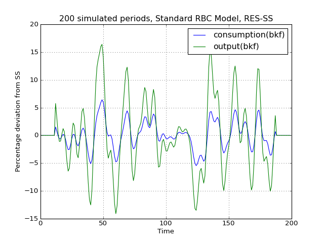
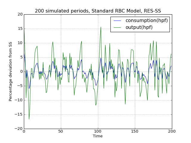
# Import the pymaclab module into its namespace, also import os module
In [1]: import pymaclab as pm
In [2]: from pymaclab.modfiles import models

# Also import matplotlib.pyplot for showing the graph
In [3]: from matplotlib import pyplot as plt

# Instantiate a new DSGE model instance like so
In [4]: rbc1 = pm.newMOD(models.stable.rbc1_res)

# Now solve and simulate the model
In [5]: rbc1.modsolvers.forkleind.solve()
In [6]: rbc1.modsolvers.forkleind.sim(200)

# Plot the simulation and show it on screen
In [7]: rbc1.modsolvers.forkleind.show_sim(('output','consumption'))
In [8]: plt.show()
This produces the following nice graph. Notice that you must specify the variables to be graphed and all simulated data is filtered according to the argument passed to each variable in the model file. So the key “hp” produces hp-filtered data, the key “bk” results in Baxter-King-filtered data while the key “cf” leads to cycles extraced using the Christiano-Fitzgerald filter.

(Source code, png, hires.png, pdf)

Cross-correlation tables¶

Notice that filtered simulations are always stored in data fields which means that statistics such as correlations at leads and lags can easily be computed as well. Specifically, the simlulated data corresponding to the above graph can be retrieved from the object rbc1.modsolver.forkleind.insim [#f1]_. There already exist a number of simple convenience functions allowing users to generate cross-correlation tables for simulated data. The functions can be used as follows:
# Import the pymaclab module into its namespace, also import os module
In [1]: import pymaclab as pm
In [2]: from pymaclab.modfiles import models

# Also import matplotlib.pyplot for showing the graph
In [3]: from matplotlib import pyplot as plt
In [4]: from copy import deepcopy

# Instantiate a new DSGE model instance like so
In [5]: rbc1 = pm.newMOD(models.stable.rbc1_res)

# Now solve and simulate the model
In [6]: rbc1.modsolvers.forkleind.solve()
In [7]: rbc1.modsolvers.forkleind.sim(200)

# Generate the cross-correlation table and show it
# Produce table with 4 lags and 4 leads using output as baseline
In [8]: rbc1.modsolvers.forkleind.mkact('output',(4,4))
In [9]: rbc1.modsolvers.forkleind.show_act()

Autocorrelation table, current output
=================================================================
productivity  |-0.016  0.109  0.335  0.663  0.997  0.619  0.264  0.034 -0.084
capital       |-0.433 -0.429 -0.381 -0.258 -0.024  0.318  0.522  0.599  0.596
consumption   |-0.134 -0.009  0.228  0.587  0.98   0.699  0.404  0.198  0.08
output        |-0.049  0.077  0.308  0.647  1.     0.646  0.305  0.08  -0.039
If users wish to obtain the data of the above table directly in order to import them into a different environment more suitable for producing publication-quality tables, the cross-correlation data can be accesssed at rbc1.modsolvers.forkleind.actm which is a matrix object of cross-correlations at the leads and lags specified in the previous calling function generating that table data.

Simulating while keeping random shocks fixed¶

Yet another useful feature to know about is that after each call to rbc1.modsolvers.forkleind.sim() the vector of randomly drawn iid shocks gets saved into object rbc1.modsolver.forkleind.shockvec. This is useful because when calling the simulation function, we can also pass an existing pre-computed vector of shocks as an argument instead of allowing the call to generate a new draw of random shocks. That way we can keep the random shocks fixed from model run to model run. So this would be accomplished as follows:
# Import the pymaclab module into its namespace, also import os module
In [1]: import pymaclab as pm
In [2]: from pymaclab.modfiles import models

# Also import matplotlib.pyplot for showing the graph
In [3]: from matplotlib import pyplot as plt
In [4]: from copy import deepcopy

# Instantiate a new DSGE model instance like so
In [5]: rbc1 = pm.newMOD(models.stable.rbc1_res)

# Now solve and simulate the model
In [6]: rbc1.modsolvers.forkleind.solve()
In [7]: rbc1.modsolvers.forkleind.sim(200)

# Plot the simulation and show it on screen
In [8]: rbc1.modsolvers.forkleind.show_sim(('output','consumption'))
In [9]: plt.show()

# Now save the shocks, by saving a clone or copy, instead of a reference
In [10]: shockv = deepcopy(rbc1.modsolvers.forkleind.shockvec)

# Now we could run the simulation again, this time passing the randomly drawn shocks
In [11]: rbc1.modsolvers.forkleind.sim(200,shockvec=shockv)

# Plot the simulation and show it on screen
In [12]: rbc1.modsolvers.forkleind.show_sim(('output','consumption'))
In [13]: plt.show()
Notice that in this script the graphs plotted to screen using the plt.show() command will produce identical graphs as the random draw of shocks only occurs in the first call to sim() while in the second it gets passed as an argument with a value retrieved and retained from the first simulation run. The reason why this feature is so useful has to do with the fact that sometimes we wish to produce summary statistics from simulation runs of one version of a model, then tweak the model’s properties dynamically at runtime and re-compute the very same summary statistics, under the assumption of holding the iid errors fixed, so that we can observe the pure net effect from changing the model’s properties elimiting any unwanted variation from “sampling variation”. As an example of this we demonstrate a script in which simulations are run and plotted under different filtering assumption.
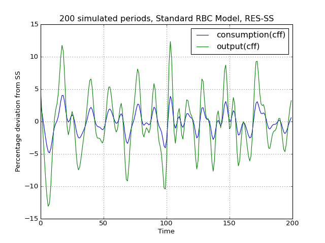
# Import the pymaclab module into its namespace, also import os module
In [1]: import pymaclab as pm
In [2]: from pymaclab.modfiles import models

# Also import matplotlib.pyplot for showing the graph
In [3]: from matplotlib import pyplot as plt
In [4]: from copy import deepcopy

# Instantiate a new DSGE model instance like so
In [5]: rbc1 = pm.newMOD(models.stable.rbc1_res,mk_hessian=False)

# Now solve and simulate the model
In [6]: rbc1.modsolvers.forkleind.solve()
In [7]: rbc1.modsolvers.forkleind.sim(200)

# Plot the simulation and show it on screen
In [8]: rbc1.modsolvers.forkleind.show_sim(('output','consumption'))
In [9]: plt.show()

# Now save the shocks, by saving a clone or copy, instead of a reference
In [10]: shockv = deepcopy(rbc1.modsolvers.forkleind.shockvec)

# Change the filtering assumption of output and consumption using the queued updater branch
In [11]: rbc1.updaters_queued.vardic['con']['mod'][0][1] = 'hp'
In [12]: rbc1.updaters_queued.vardic['con']['mod'][1][1] = 'hp'
In [13]: rbc1.updaters_queued.process_queue()

# Now we could run the simulation again, this time passing the randomly drawn shocks
In [14]: rbc1.modsolvers.forkleind.solve()
In [15]: rbc1.modsolvers.forkleind.sim(200,shockvec=shockv)

# Plot the simulation and show it on screen
In [16]: rbc1.modsolvers.forkleind.show_sim(('output','consumption'))
In [17]: plt.show()

# Change the filtering assumption of output and consumption using the queued updater branch
In [18]: rbc1.updaters_queued.vardic['con']['mod'][0][1] = 'cf'
In [19]: rbc1.updaters_queued.vardic['con']['mod'][1][1] = 'cf'
In [20]: rbc1.updaters_queued.process_queue()

# Now we could run the simulation again, this time passing the randomly drawn shocks
In [21]: rbc1.modsolvers.forkleind.solve()
In [22]: rbc1.modsolvers.forkleind.sim(200,shockvec=shockv)

# Plot the simulation and show it on screen
In [23]: rbc1.modsolvers.forkleind.show_sim(('output','consumption'))
In [24]: plt.show()
(Source code, png, hires.png, pdf)

(png, hires.png, pdf)

(png, hires.png, pdf)

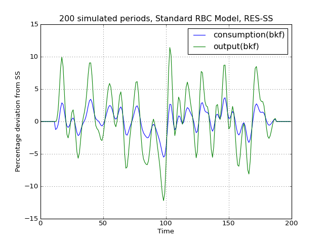
As is apparent from the three plots produced above, the simulated data is first filtered using the Baxter-King filter, then the more commonly used Hodrick-Prescott filter and finally the Christian-Fitzgerald asymmetric filter. Notice that the BK filter by default (or rather by specification) cuts off 6 time periods at the beginning and at the end of the simulated sample. The purpose for using any of the three filters is of course to make the simulated data stationary and to extract the cycle only.

Generating impulse-response functions¶

Dynamic solutions obtained to first-order approximated DSGE models using the method of perturbations have a great deal in common with standard Vector Autoregression (VAR) models commonly used in applied Macroeconometrics. This in turn implies that solved DSGE models can be described using so-called impulse-response functions (also abbreviated as IRFs) or impulse-response graphs which show how the solved model responds to a one-off shock to a particular exogenous state variable. In PyMacLab this can easily be achieved as follows:
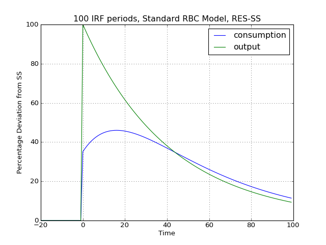
# Import the pymaclab module into its namespace, also import os module
In [1]: import pymaclab as pm
In [2]: from pymaclab.modfiles import models

# Also import matplotlib.pyplot for showing the graph
In [3]: from matplotlib import pyplot as plt

# Instantiate a new DSGE model instance like so
In [4]: rbc1 = pm.newMOD(models.stable.rbc1_res)

# Now solve and simulate the model
In [5]: rbc1.modsolvers.forkleind.solve()
In [6]: rbc1.modsolvers.forkleind.irf(100,('productivity',))

# Plot the simulation and show it on screen
In [7]: rbc1.modsolvers.forkleind.show_irf(('output','consumption'))
In [8]: plt.show()
This produces the following nice graph. Notice that here the shock to total productivity has been normalized to 100%.

(Source code, png, hires.png, pdf)

Footnotes

[4] The simulated time series data contained within rbc1.modsolvers.forkleind.insim is NOT filtered yet. In designing the library I have decided to delay filtering to the stage where the user calls rbc1.modsolvers.forkleind.show_sim() or when similar functions are called to for instance generate the cross-correlation table.

PyMacLab Tutorial Series¶

Tutorial 1 - Getting started¶

Introduction¶

Tutorial 3 - The PyMacLab DSGE instance¶

Introduction¶

Understanding the PyMacLab DSGE model class and its instances¶

Instantiation options for DSGE model instances¶

Working with DSGE model instances¶

DSGE modelling made intuitive¶

Tutorial 4 - The Python DSGE instance updater methods¶

Introduction¶

One-off alteration of one specific model property¶

Altering many model properties and queued processing¶

Tutorial 5 - Steady State Solution Methods¶

Introduction¶

Option 1: Using the model’s declared FOCs and passing arguments at model instantiation¶

Option 2: Using the model’s declared FOCs and passing arguments inside the model file¶

Option 3: Supplying the non-linear steady state system in the model file¶

Option 4: Use the numerical root finder to solve for some steady states and get remaining ones residually¶

Option 5: Use the numerical root finder to solve for steady states with pre-computed starting values¶

Option 6: Computing the steady state values dictionary entirely outside of PyMacLab and passing it¶

Option 7: Finding the steady state by only supplying information in the Closed Form section¶

More about the steady state and its relevance to perturbation methods - A Detour¶

Tutorial 6 - Dynamic Solution Methods¶

Introduction¶

The Jacobian and Hessian: A Detour¶

Dynamic Solution Methods - Nth-order Perturbation¶

Choosing the degree of approximation¶

Tutorial 7 - Simulating DSGE models¶

Introduction¶

Simulating the model¶

Cross-correlation tables¶

Simulating while keeping random shocks fixed¶

Generating impulse-response functions¶

Table Of Contents

Previous topic

Next topic

This Page

Option with default value	Description
`pm.newMOD(mpath,initlev=2)`	Initlev=0 only parses and prepares for manual steady state calculation
	Initlev=1 does initlev=0 and attempts to solve for the model’s steady state automatically
	Initlev=2 does initlev=0, initlev=1 and generates Jacobian and Hessian and solves model dynamically
`pm.newMOD(mpath,mesg=False)`	Prints very useful runtime instantiation messages to the screen for users to follow progress
`pm.newMOD(mpath,ncpus=1)`	CPU cores to be used in expensive computation of model’s derivatives, ‘auto’ for auto-detection
`pm.newMOD(mpath,mk_hessian=True)`	Should Hessian be computed at all, as is expensive?
`pm.newMOD(mpath,use_focs=False)`	Should only the model’s FOCs be used to computed the steady state? Accepts Python list or tuple
`pm.newMOD(mpath,ssidic=None)`	Use in conjunction with previous argument to specify initial starting values as Python dictionary
`pm.newMOD(mpath,sstate=None)`	Specify steady state values as Python dictionary and supply here. No SS computation in instance

Wrapped updater object	Description
`model.updaters.paramdic`	Inserting updated values re-initializes the model with new set of parameter values
`model.updaters.vardic`	Inserting new values updates/changes values and attributes defined for variables used in the model
`model.updaters.nlsubsdic`	Inserting new values updates the dictionary of variable substitution items beginning with @
`model.updaters.foceqs`	Inserting new string equations updates the set of non-linear first-order conditions of optimality
`model.updaters.manss_sys`	In this list users can insert new equations as strings into the closed form steady state system
`model.updaters.ssys_list`	In this list users can insert new equations as strings into the numerical steady state system
`model.updaters.sigma`	A wrapped matrix which updates the model when changed values are inserted in the varcovar-matrix

Wrapped updater object	Description
`model.updaters_queued.paramdic`	Inserting updated values re-initializes the model with new set of parameter values
`model.updaters_queued.vardic`	Inserting new values updates/changes values and attributes defined for variables used in the model
`model.updaters_queued.nlsubsdic`	Inserting new values updates the dictionary of variable substitution items beginning with @
`model.updaters_queued.foceqs`	Inserting new string equations updates the set of non-linear first-order conditions of optimality
`model.updaters_queued.manss_sys`	In this list users can insert new equations as strings into the closed form steady state system
`model.updaters_queued.ssys_list`	In this list users can insert new equations as strings into the numerical steady state system
`model.updaters_queued.sigma`	A wrapped matrix which updates the model when changed values are inserted in the varcovar-matrix
`model.updaters_queued.queue`	The actual queue. Here objects which have been altered will be stored as strings
`model.updaters_queued.process_queue`	The queue processing method which finally updates the queued objects in the right order

Object	Description
`rbc1.modsolvers.forkleind.P`	Matrix of elasticities describing optimal law of motion for endog. state variables, 1st-order part
`rbc1.modsolvers.forkleind.F`	Matrix of elasticities describing optimal law of motion for endog. state variables, 1st-order part
`rbc1.modsolvers.forkleind.G`	Matrix of elasticities describing optimal law of motion for endog. state variables, 2nd-order part
`rbc1.modsolvers.forkleind.E`	Matrix of elasticities describing optimal law of motion for endog. state variables, 2nd-order part
`rbc1.modsolvers.forkleind.KX`	Array of risk-adjustment values for steady states of endogenous state variables
`rbc1.modsolvers.forkleind.KY`	Array of risk-adjustment values for steady states of control variables

Navigation

PyMacLab Tutorial Series¶

Tutorial 1 - Getting started¶

Introduction¶

Tutorial 3 - The PyMacLab DSGE instance¶

Introduction¶

Understanding the PyMacLab DSGE model class and its instances¶

Instantiation options for DSGE model instances¶

Working with DSGE model instances¶

DSGE modelling made intuitive¶

Tutorial 4 - The Python DSGE instance updater methods¶

Introduction¶

One-off alteration of one specific model property¶

Altering many model properties and queued processing¶

Tutorial 5 - Steady State Solution Methods¶

Introduction¶

Option 1: Using the model’s declared FOCs and passing arguments at model instantiation¶

Option 2: Using the model’s declared FOCs and passing arguments inside the model file¶

Option 3: Supplying the non-linear steady state system in the model file¶

Option 4: Use the numerical root finder to solve for some steady states and get remaining ones residually¶

Option 5: Use the numerical root finder to solve for steady states with pre-computed starting values¶

Option 6: Computing the steady state values dictionary entirely outside of PyMacLab and passing it¶

Option 7: Finding the steady state by only supplying information in the Closed Form section¶

More about the steady state and its relevance to perturbation methods - A Detour¶

Tutorial 6 - Dynamic Solution Methods¶

Introduction¶

The Jacobian and Hessian: A Detour¶

Dynamic Solution Methods - Nth-order Perturbation¶

Choosing the degree of approximation¶

Tutorial 7 - Simulating DSGE models¶

Introduction¶

Simulating the model¶

Cross-correlation tables¶

Simulating while keeping random shocks fixed¶

Generating impulse-response functions¶

Table Of Contents

Previous topic

Next topic

This Page

Quick search

Navigation