Tutorial 7 - Simulating DSGE models
Introduction
In the previous tutorial we discovered the general structure of the PyMacLab DSGE model instance and saw how this programming approach lent itself well to the idea of inspecting and exploring the instantiated models’ current state, summarized by its data fields and supplied instance methods equipping them with functionality. This section finally discusses how the library equips DSGE model instances with methods which make use of the models’ computed Jacobian and Hessian, which are evaluated at the models’ numerical steady state. As a short reminder, we may recall here that it is often this step of obtaining a steady state can prove difficult in the case of a number of well-known models. Notwithstanding, for the remainder of this section we will assume that a steady state has successfully been attained and that the model’s Jacobian and Hessian have been computed. Let’s first start with our usual setup of lines of code entered into an IPython shell:
# Import the pymaclab module into its namespace, also import os module
In [1]: import pymaclab as pm
In [2]: from pymaclab.modfiles import models

# Instantiate a new DSGE model instance like so
In [4]: rbc1 = pm.newMOD(models.stable.rbc1_res)
Simulating the model
Recall that instantiating a DSGE model without any additional parameters means that an automatic attempt of finding the steady state is being made and if successfully found the model is already solved dynamically using a preferred (1st-order approximate) method. This means that you now have all the information you need to simulate the model as well as to generate impulse-response functions and plot them. Let’s focus on the simulations first, they are being generate using the following command:
# Import the pymaclab module into its namespace, also import os module
In [1]: import pymaclab as pm
In [2]: from pymaclab.modfiles import models

# Instantiate a new DSGE model instance like so
In [3]: rbc1 = pm.newMOD(models.stable.rbc1_res)

# Now simulate the model
In [4]: rbc1.modsolvers.forkleind.sim(200,('productivity'))
This would simulate the model for 200 time periods using only iid shocks hitting the law of motion of the total factor productivity term in the model. Notice that here RBC1 is a very simple model only containing one structural shock, but more complicated models may possess more than one exogenous state variable. In that case, if you called instead:
# Import the pymaclab module into its namespace, also import os module
In [1]: import pymaclab as pm
In [2]: from pymaclab.modfiles import models

# Instantiate a new DSGE model instance like so
In [3]: rbc1 = pm.newMOD(models.stable.rbc1_res)

# Now simulate the model
In [4]: rbc1.modsolvers.forkleind.sim(200)
The model would be simulated using all shocks (exogenous state variables) specified in the model. However, since rbc1 only contains one shock, the two variants shown here of simulating the model would yield the same results as “productivity” is is the only exogenous state available here anyway. We can then also graph the simulation to get a better understanding of the model by running the command:
# Import the pymaclab module into its namespace, also import os module
In [1]: import pymaclab as pm
In [2]: from pymaclab.modfiles import models

# Also import matplotlib.pyplot for showing the graph
In [3]: from matplotlib import pyplot as plt

# Instantiate a new DSGE model instance like so
In [4]: rbc1 = pm.newMOD(models.stable.rbc1_res)

# Now solve and simulate the model
In [5]: rbc1.modsolvers.forkleind.solve()
In [6]: rbc1.modsolvers.forkleind.sim(200)

# Plot the simulation and show it on screen
In [7]: rbc1.modsolvers.forkleind.show_sim(('output','consumption'))
In [8]: plt.show()
This produces the following nice graph. Notice that you must specify the variables to be graphed and all simulated data is filtered according to the argument passed to each variable in the model file. So the key “hp” produces hp-filtered data, the key “bk” results in Baxter-King-filtered data while the key “cf” leads to cycles extraced using the Christiano-Fitzgerald filter.
(Source code, png, hires.png, pdf)
Cross-correlation tables
Notice that filtered simulations are always stored in data fields which means that statistics such as correlations at leads and lags can easily be computed as well. Specifically, the simlulated data corresponding to the above graph can be retrieved from the object rbc1.modsolver.forkleind.insim [1]. There already exist a number of simple convenience functions allowing users to generate cross-correlation tables for simulated data. The functions can be used as follows:
# Import the pymaclab module into its namespace, also import os module
In [1]: import pymaclab as pm
In [2]: from pymaclab.modfiles import models

# Also import matplotlib.pyplot for showing the graph
In [3]: from matplotlib import pyplot as plt
In [4]: from copy import deepcopy

# Instantiate a new DSGE model instance like so
In [5]: rbc1 = pm.newMOD(models.stable.rbc1_res)

# Now solve and simulate the model
In [6]: rbc1.modsolvers.forkleind.solve()
In [7]: rbc1.modsolvers.forkleind.sim(200)

# Generate the cross-correlation table and show it
# Produce table with 4 lags and 4 leads using output as baseline
In [8]: rbc1.modsolvers.forkleind.mkact('output',(4,4))
In [9]: rbc1.modsolvers.forkleind.show_act()

Autocorrelation table, current output
=================================================================
productivity  |-0.016  0.109  0.335  0.663  0.997  0.619  0.264  0.034 -0.084
capital       |-0.433 -0.429 -0.381 -0.258 -0.024  0.318  0.522  0.599  0.596
consumption   |-0.134 -0.009  0.228  0.587  0.98   0.699  0.404  0.198  0.08
output        |-0.049  0.077  0.308  0.647  1.     0.646  0.305  0.08  -0.039
If users wish to obtain the data of the above table directly in order to import them into a different environment more suitable for producing publication-quality tables, the cross-correlation data can be accesssed at rbc1.modsolvers.forkleind.actm which is a matrix object of cross-correlations at the leads and lags specified in the previous calling function generating that table data.
Simulating while keeping random shocks fixed
Yet another useful feature to know about is that after each call to rbc1.modsolvers.forkleind.sim() the vector of randomly drawn iid shocks gets saved into object rbc1.modsolver.forkleind.shockvec. This is useful because when calling the simulation function, we can also pass an existing pre-computed vector of shocks as an argument instead of allowing the call to generate a new draw of random shocks. That way we can keep the random shocks fixed from model run to model run. So this would be accomplished as follows:
# Import the pymaclab module into its namespace, also import os module
In [1]: import pymaclab as pm
In [2]: from pymaclab.modfiles import models

# Also import matplotlib.pyplot for showing the graph
In [3]: from matplotlib import pyplot as plt
In [4]: from copy import deepcopy

# Instantiate a new DSGE model instance like so
In [5]: rbc1 = pm.newMOD(models.stable.rbc1_res)

# Now solve and simulate the model
In [6]: rbc1.modsolvers.forkleind.solve()
In [7]: rbc1.modsolvers.forkleind.sim(200)

# Plot the simulation and show it on screen
In [8]: rbc1.modsolvers.forkleind.show_sim(('output','consumption'))
In [9]: plt.show()

# Now save the shocks, by saving a clone or copy, instead of a reference
In [10]: shockv = deepcopy(rbc1.modsolvers.forkleind.shockvec)

# Now we could run the simulation again, this time passing the randomly drawn shocks
In [11]: rbc1.modsolvers.forkleind.sim(200,shockvec=shockv)

# Plot the simulation and show it on screen
In [12]: rbc1.modsolvers.forkleind.show_sim(('output','consumption'))
In [13]: plt.show()
Notice that in this script the graphs plotted to screen using the plt.show() command will produce identical graphs as the random draw of shocks only occurs in the first call to sim() while in the second it gets passed as an argument with a value retrieved and retained from the first simulation run. The reason why this feature is so useful has to do with the fact that sometimes we wish to produce summary statistics from simulation runs of one version of a model, then tweak the model’s properties dynamically at runtime and re-compute the very same summary statistics, under the assumption of holding the iid errors fixed, so that we can observe the pure net effect from changing the model’s properties elimiting any unwanted variation from “sampling variation”. As an example of this we demonstrate a script in which simulations are run and plotted under different filtering assumption.
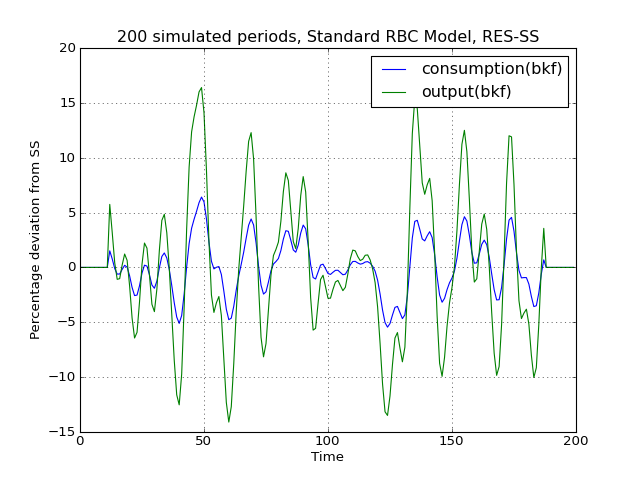
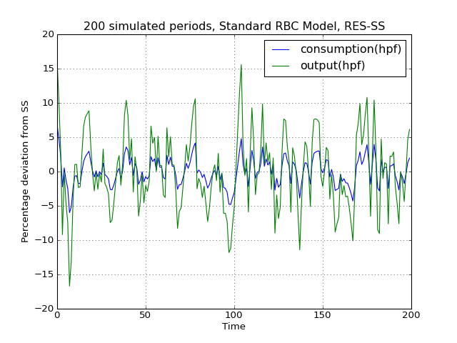
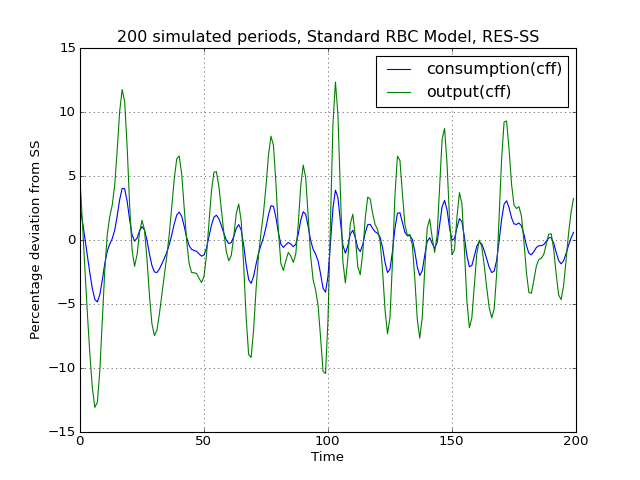
# Import the pymaclab module into its namespace, also import os module In [1]: import pymaclab as pm In [2]: from pymaclab.modfiles import models # Also import matplotlib.pyplot for showing the graph In [3]: from matplotlib import pyplot as plt In [4]: from copy import deepcopy # Instantiate a new DSGE model instance like so In [5]: rbc1 = pm.newMOD(models.stable.rbc1_res,mk_hessian=False) # Now solve and simulate the model In [6]: rbc1.modsolvers.forkleind.solve() In [7]: rbc1.modsolvers.forkleind.sim(200) # Plot the simulation and show it on screen In [8]: rbc1.modsolvers.forkleind.show_sim(('output','consumption')) In [9]: plt.show() # Now save the shocks, by saving a clone or copy, instead of a reference In [10]: shockv = deepcopy(rbc1.modsolvers.forkleind.shockvec) # Change the filtering assumption of output and consumption using the queued updater branch In [11]: rbc1.updaters_queued.vardic['con']['mod'][0][1] = 'hp' In [12]: rbc1.updaters_queued.vardic['con']['mod'][1][1] = 'hp' In [13]: rbc1.updaters_queued.process_queue() # Now we could run the simulation again, this time passing the randomly drawn shocks In [14]: rbc1.modsolvers.forkleind.solve() In [15]: rbc1.modsolvers.forkleind.sim(200,shockvec=shockv) # Plot the simulation and show it on screen In [16]: rbc1.modsolvers.forkleind.show_sim(('output','consumption')) In [17]: plt.show() # Change the filtering assumption of output and consumption using the queued updater branch In [18]: rbc1.updaters_queued.vardic['con']['mod'][0][1] = 'cf' In [19]: rbc1.updaters_queued.vardic['con']['mod'][1][1] = 'cf' In [20]: rbc1.updaters_queued.process_queue() # Now we could run the simulation again, this time passing the randomly drawn shocks In [21]: rbc1.modsolvers.forkleind.solve() In [22]: rbc1.modsolvers.forkleind.sim(200,shockvec=shockv) # Plot the simulation and show it on screen In [23]: rbc1.modsolvers.forkleind.show_sim(('output','consumption')) In [24]: plt.show()(Source code, png, hires.png, pdf)
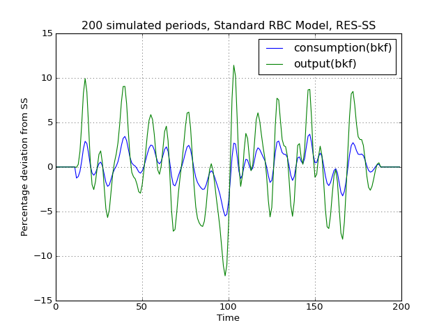
As is apparent from the three plots produced above, the simulated data is first filtered using the Baxter-King filter, then the more commonly used Hodrick-Prescott filter and finally the Christian-Fitzgerald asymmetric filter. Notice that the BK filter by default (or rather by specification) cuts off 6 time periods at the beginning and at the end of the simulated sample. The purpose for using any of the three filters is of course to make the simulated data stationary and to extract the cycle only.
Generating impulse-response functions
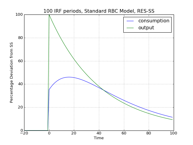
Dynamic solutions obtained to first-order approximated DSGE models using the method of perturbations have a great deal in common with standard Vector Autoregression (VAR) models commonly used in applied Macroeconometrics. This in turn implies that solved DSGE models can be described using so-called impulse-response functions (also abbreviated as IRFs) or impulse-response graphs which show how the solved model responds to a one-off shock to a particular exogenous state variable. In PyMacLab this can easily be achieved as follows:
# Import the pymaclab module into its namespace, also import os module
In [1]: import pymaclab as pm
In [2]: from pymaclab.modfiles import models

# Also import matplotlib.pyplot for showing the graph
In [3]: from matplotlib import pyplot as plt

# Instantiate a new DSGE model instance like so
In [4]: rbc1 = pm.newMOD(models.stable.rbc1_res)

# Now solve and simulate the model
In [5]: rbc1.modsolvers.forkleind.solve()
In [6]: rbc1.modsolvers.forkleind.irf(100,('productivity',))

# Plot the simulation and show it on screen
In [7]: rbc1.modsolvers.forkleind.show_irf(('output','consumption'))
In [8]: plt.show()
This produces the following nice graph. Notice that here the shock to total productivity has been normalized to 100%.
(Source code, png, hires.png, pdf)
Footnotes
| [1] | The simulated time series data contained within rbc1.modsolvers.forkleind.insim is NOT filtered yet. In designing the library I have decided to delay filtering to the stage where the user calls rbc1.modsolvers.forkleind.show_sim() or when similar functions are called to for instance generate the cross-correlation table. |
